
How to Be Awesome at Biostatistics and Literature Evaluation - Part I
Raise your hand if you like evaluating clinical research.

Aww come on, really? You don't like calling shenanigans on a sneaky study for reporting relative risk while ignoring absolute risk?

Okay, okay. Fine.
But like it or not, biostats isn't going away. I've been asked by a surprising number of students over the years why they "need" to learn stats. It's usually with some variation of the phrase "I already have a job lined up with VCS Community Pharmacy, stats have no part in my day there."
Fair objection. My counter argument is usually multi-tiered:
You may not want to work at VCS forever. It's really hard to predict your 5 or 10 year situation with a field that changes as often as pharmacy
Even at VCS, you're going to be dispensing a huge number of the new drugs that come out. Patients will ask you about them. Knowing the data that got the drug approved can help you counsel for side effects and make informed decisions about cost/benefit. If you only see yourself as a "pill counter" that's all you will be (and pill counters are replaceable).
You're going to finish up your 4 professional years with a doctoral degree. People will call you "doctor." A doctor in any field is recognized as someone that can think critically and interpret data within their profession. Literature evaluation teaches critical thinking and data interpretation. You're living in a dream world if you think ACPE will say "buh bye" to that part of the curriculum.
Complaining about biostatistics doesn't change the fact that you have a test later this week. You should probably get studying.
So if biostats and literature evaluation are here to stay, we may as well become friends with them. You don't have to send them a Christmas card or anything, but you should at least give them the cursory "Happy Birthday" message on Facebook.
This post is Part I of a 4-part series. But it can serve as your one stop shop for all things biostats and clinical literature. I can't get you from A to Z, but I can get you from A to K (which is right around "I'm not an expert, but I know enough to be dangerous" territory). You'll have a working knowledge that you can build on.
And if you understand everything in this post, you should do just fine on your test next week.
I'll start by breaking down the basic terms and concepts in biostatistics. Then we'll talk about the types of statistical tests (and when and when not to use them). Then we're gonna drop the hammer on literature evaluation. I want to keep this practical, so I'll primarily focus on decoding some of the "tricks" commonly used to make a study look better than it is.
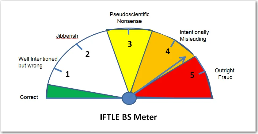
By the end of this series, your BS Meters should be finely tuned and ready for action.
If you’d like, you can get this entire series (Parts I - IV) consolidated into a single printer-friendly and savable PDF. It’s perfect for offline viewing. You can find that here.

Biostatistics Terms and Concepts
There's no easy way to segue into this, so let's just dive right in.
Descriptive vs Inferential Statistics
There are two main branches of statistics used in clinical literature evaluation; descriptive and inferential. They're both exactly what they sound like. Descriptive statistics "describe" something. Inferential statistics "infer" (aka predict) something.
Put another way, descriptive statistics use data to describe the study population. For example, we might take a given patient population and say that it has a mean (average) age of 57.
Inferential statistics use data to make predictions about the population. This is most frequently used to "generalize" an observation about a study group to the overall population. For example, if I wanted to know the rate of depression in American pharmacy students, it's not realistic for me to get data from every student in the country. So instead, I could tally the rate of depression at a handful of pharmacy schools and extrapolate that data to the general population of "American pharmacy students."
Doesn't that open the door for a ton of potential fallacies, errors, and biases? You bet.
And it's important to keep that in mind with every single paper that you read. Almost all clinical studies use some form of inferential statistics. It's not that they're "wrong" or "bad." It's literally impossible (not to mention impractical) to measure the entire population for a given disease state. Inferences have to be made.
But those inferences are what led Mark Twain to famously quip:
"There are lies, damned lies, and statistics."
- Mark Twain
So it's really just about preparing yourself for this reality beforehand and approaching every study you read with a certain level of scrutiny.
Types of Data
I'm about to set a record for how often I use the word "data" in a few paragraphs. So lets first clarify what I mean by data.
There are two main "branches" on the tree of data, quantitative and qualitative. Qualitative data involves descriptive things that don't have any numeric value. When you fill out a class evaluation survey every semester, and you're asked to write out "What suggestions do you have to improve this class?", you're filling out qualitative data. There's no way to "rank" your response compared to your classmates.
Qualitative data can be useful (I use it all the time to improve articles and products at tl;dr pharmacy), but it's not where we're going to focus in this article. You're not going to come across it that frequently in a clinical study, because it can be inherently subjective. Qualitative data often involves someone's perception of some experience. When we're making decisions on whether to give a drug to someone or not, we want objective data to guide that decision.
The family tree of quantitative data gets broken down to the two main categories of discrete and continuous.

And as you can see from the picture above, discrete and continuous data are further broken down into more sub-categories.
Continuous data can be either interval or ratio.
Interval Data - Has a meaningful numeric value. The difference between 2 consecutive values is consistent along the scale. However, there is no "real" zero point. It's arbitrary.
A common example used to illustrate interval data is the Celsius temperature scale. Higher temperatures are always "hotter" than lower temperatures. But 0 degrees Celsius doesn't really mean anything, because there are negative Celsius temperatures. Even still, the scale is always consistent. 0 degrees is exactly 20 degrees warmer than -20 degrees. 50 degrees is exactly 20 degrees warmer than 30 degrees. And so on.
Ratio Data - Is the same thing as interval data, except that it has a meaningful zero point. The Kelvin temperature scale is ratio data, because there is an absolute zero (there are no negative degrees Kelvin). Other examples of ratio data are weight and length.
Rule of thumb: If you need to break an established law of Physics to have a negative value (e.g. someone weighing -86 kg), then it's ratio data.
One final point is that continuous data can include decimal points and other non-integers. So if the data point you're looking at is 16.57, then it's continuous data.
Let's move on to discrete data. Don't let the fact that it is "quantitative" fool you. Discrete data describes types of data that are mutually exclusive (i.e. discrete) from each other. For example, you cannot be both 28 years old and 35 years old. Being one age precludes you from being another.
How does this turn out to be quantitative? Because we use it to count up or tally information about participants in a study. For example, we can use discrete data to determine that there are 348 females and 352 males in a study population. We can also use discrete data to further categorize our study population by age, gender, or some marker for their disease state (such as the NYHA functional class staging for heart failure).
Discrete data is broken up into nominal, ordinal, and binary.
Nominal Data - Generally speaking, is used for things with no numeric value. Things like ethnicity and marital status fit here. They have no inherent quantitative meaning.
Binary Data - A special class of discrete data with only two options. The classic example of binary data is gender (although depending on the study population, gender may no longer be binary). Binary data is often lumped together with nominal data. In fact, depending on your school's curriculum, you may not even learn about this special subcategory. That's not "wrong," but my inner math nerd won't be happy unless I give binary data some cred here.
Ordinal Data - Has a ranking system to it, unlike nominal data. Here, the ranking order is important. That NYHA functional staging for heart failure we mentioned a few paragraphs ago is ordinal data. Class III heart failure is worse than Class I heart failure. However (and this is important), unlike continuous data, the difference between the ranked classes is not equal. So, for example, Class IV heart failure is not twice as bad as Class II heart failure. This is different from continuous data, where 40 degrees Celsius is exactly 5 degrees colder than 45 degrees. Other examples of ordinal data may be cancer staging, Apgar scores, and pretty much anything using a Likert scale.
Before we move on from types of data, here's a couple of common tripping points. First, remember that discrete data can only be whole numbers (integers). If there's any sort of a decimal, then you're dealing with continuous data. This makes Age a common discrete data point, because we don't usually say that someone is 34.65 years old. In most clinical studies, you're either 34, or you're 35.
Another point; we can convert one type of data into another. For example, we can take the nominal data of "Age" and convert it to ordinal by assigning categories. We could break the age of the study population into 4 categories, for example:
Age: < 20 years old
Age: 20 - 40 years old
Age: 41 - 60 years old
Age: > 60 years old
Classifying this way puts it an order where rank is important (and so it's ordinal).
Similarly, we can convert qualitative data into quantitative. For instance, if you purchase Mastering the Match from tl;dr pharmacy, you're eventually going to get an email from me where I ask you for feedback. I then take those responses and group them into categories. Essentially, I've just made nominal data from qualitative responses. I then use that data to improve the next edition of the book.
Big Ole List of Biostats Terms

Here's your teaser. You're gonna want to click the link to the left to see Anger Dancing in all its majesty. (Image credit)
A quick preface for this section: I am not usually a big fan of throwing giant lists of terms together with no context. It's sort of a cop out by the writer, and it doesn't teach the reader as much as it could. If I click a link claiming to be an "Ultimate Guide" on something, and all I see is an outline of someone's personal notes, it gets me mad enough to "Anger Dance" like Kevin Bacon in the movie Footloose.
That being said, what follows is exactly such a list. I'll provide as much context as I can, but I'm writing this section assuming that you have at least a cursory understanding of biostats. You should have at least seen these terms before...and I don't want to get into a breakdown of the X versus Y axis.
An entire post could literally be dedicated to every one of the following terms. What will follow here is just an overview. As always, if you have follow up questions, email me at mail@tldrpharmacy.com and I will try to clarify. If enough people need further clarification, perhaps one day I will make a separate mini-post for each term.
Dependent Variable
The outcome of interest. This variable "depends" on the intervention. For example, we could compare atorvastatin versus placebo to see if it has an impact on the number of secondary ASCVD events. The dependent variable (i.e. the thing we care about) here is the number of secondary ASCVD events. We're testing the likelihood that secondary ASCVD events depend on whether or not a patient takes atorvastatin.
Independent Variable
The intervention. The thing we're actually manipulating. In our example above, the independent variable is atorvastatin. It doesn't "depend" on any other event.
Population
The entire population you're interested in. Using our example above, "All patients with a prior ASCVD event" would be our population. Take special note that this is the entire population. The entire population is usually too cumbersome to study, so instead we use a...
Sample
Also known as "Study Population."A subset of the population taken because the entire population is too large to analyze. The characteristics of the sample are supposed to be representative of the population.
Side Note: This is an important red flag to look out for when analyzing a study. Certain demographics (e.g. Caucasian males) are often over-represented in clinical trials. When a study uses a sample to represent the overall population, your job is to make sure that sample is an accurate representation.
Mean
The average value of a sample distribution. You add up everything in a list, and divide by the total number of values:
Mean = sum of all values / number of values
There's a "weakness" to the mean. It's sensitive to outliers. It can be affected by "skews" or aberrations in the data. For example...if I were to take the mean of the following 4 numbers...
4, 12, 8, 100
...then the mean would be 31
Does 31 sound like a fair representation of the sample population considering that 3 of the numbers are 12 or less?
One last bit about the mean: It can only be used for continuous data. This makes intuitive sense if you think about it. If we were to look at a patient population with heart failure, we couldn't take the "average" NYHA class of heart failure of the population. Our study population might end up with an average NYHA class of 2.3...and what the hell does that mean? As we mentioned above, NYHA classification of heart failure is ordinal (not continuous) data, so a mean does not apply.
Median
The value in the middle of the list. You take the data points and arrange them in numerical order from lowest to highest. Then, the number in the middle of that data is the median. You're left with a situation where half of the data is larger than the median, and half is smaller. If you have an even number of observations, then you take the two middle numbers and average them.
So with our 4 number data set above, we'd first arrange them in numeric order:
4, 8, 12, 100
Since it's an even number of data points, we'd add together the 2 middle numbers and divide by two (in effect, we're taking the mean of the 2 middle numbers).
So (8 + 12) / 2 = 10.
So while the mean of our data set was 31, the median is 10. This is the strength of the median. When there is a skewed data set (i.e. when outliers exist), the median may be a more appropriate measure. It can be used with both continuous and ordinal data.
Mode
The number that occurs most frequently in a data set. There's not a lot else to say here. The mode can be used with both continuous and ordinal data.
Range
Exactly what it sounds like. The difference between the highest and lowest values. It's a useful number, because it can set limits to an expectation of effect. You can get the upper and lower values for a given intervention. Let's say we measure a baseline % LDL for 1000 people, and then we give them 20 mg of atorvastatin for 3 months. After 3 months, we re-measure their % LDL. If the highest reduction was 40%, and the lowest was 5%, then our range is 35%. This is also a measurement of how precise or consistent a data set is. A large range means that the effects of our intervention can vary greatly between individuals. A small range means that we can predict with reasonable certainty the effect of our intervention.
Big Ole List of Biostats Terms: Continued
Alright, we've covered the basics on data and populations. Let's now move on to how that data is distributed and how we can visualize it (don't worry, there's pictures!).

Normal Distribution
A really smart dude named Carl Friedrich Gauss was a German mathematician who did more for math than I'll ever understand. Among the many (many) things he discovered were probabilities of distribution. Here's how it applies to your life...
According to the central limit theorem, the averages of random variables drawn from independent distributions converge to "normal," assuming the data size is large enough. In plain english, that means that if your sample size is large enough, your population will form a Gaussian (or "Normal") Distribution. This is also commonly known as a Bell Curve, because that's what it looks like on a graph. It turns out that most populations (for just about anything) will form a normal distribution. The graph above could represent IQ scores, or the people that achieved a 20% reduction in LDL from atorvastatin, or even the people that experienced myopathy as a side effect of atorvastatin.
For our purposes in clinical research, when a study population is large enough, the distribution usually approximates a normal distribution. The mean, median, and mode are all the same value, and they're right in the middle of the graph at the 50th percentile. The curve is also symmetric around the mean/median/mode. There's no "skew" to either side (I'll cover that in a bit). It's important to note that a study population has to be large enough. If you're studying an ultra rare disease and only have a patient population of 17 people, you probably will not have a normal distribution. And because we're dealing with a mean, that means (do you see what I did there?) that our data has to be continuous to form a normal distribution. Ordinal data need not apply.
Standard Deviation
You'll see this called a "measure of spread." You'll see it called "variation" or "dispersion." They all mean the same thing. Standard deviation looks at how spread out your data is. If you have a low (or small) standard deviation, your data is tightly clustered around the mean. Obviously the inverse is also true; if you have a high standard deviation, your data is more spread out. How do you apply this? Let's go back to our trusty atorvastatin intervention. If we're measuring the ability of atorvastatin to lower LDL by 20%, and the standard deviation is small, that means that the vast majority of patients will achieve that goal 20% reduction. If the standard deviation is larger, then a smaller number of patients will have the effect.
And then, tying it together, see that in a normal distribution, +/- 1 standard deviation from the mean contains about 68% of the population. Move out to 2 standard deviations, and you're dealing with 95% of the population. So in a drug study (like our atorvastatin example above), we can use standard deviation to predict the likelihood of how many patients will experience the treatment effect. Smaller standard deviation means more patients will achieve the effect.
Let's zoom back out to make sure you see the big picture here. If you're a student, there's an easy test question buried in the above paragraphs; standard deviation can only be used for continuous data in a normal distribution. If you see a multiple choice question using the standard deviation in another way, that answer is wrong.
Skewness
Not all data is normally distributed. Sometimes the bell curve is more like a rolling wave crashing into a breaker. Data sets can be positively or negatively skewed. The "skew" goes in the direction of the tail of the data, not the bulky hump.
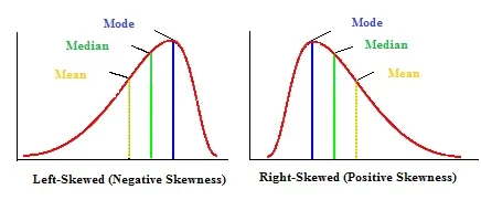
Notice that unlike our normal distribution, the mean, median, and mode are not all equal. You'll see the mode in the hump (because it's the most common data point), and then as you go off through the tail you'll see the median and then the mean. I'll just point out again that because skewed data is not normally distributed, you cannot use standard deviation to help describe it.
Null Hypothesis
This states that there is no difference between treatment groups in a study. So if we were to design a study that tests paroxetine versus placebo in treating major depressive disorder; the null hypothesis would be that paroxetine would be no better than placebo. As a general default setting, most studies start out by "assuming" the null hypothesis is true; and it's the job of the data to prove otherwise. This "innocent until proven guilty" approach helps to remove a potential bias, because something in our human brains wants and expects the null hypothesis to be false. If we've gotten far enough along that we're testing paroxetine for depression, of course we expect it to be better than a sugar pill. By setting up the statistical burden to assume there is no difference between treatment groups, we help to overcome this natural bias (and prevent ourselves from committing a Type I error, which I'll cover in a bit).
The terminology is kind of weird and "lawyer-speak" here. I'm not sure why we make it so confusing on ourselves and others. But when we discuss the results of a study, we don't "reject" the null hypothesis; we "fail to accept" it. Maybe this is to soften the blow so that the null hypothesis doesn't feel bad about itself? It's kind of like saying "It's not you, it's me...I failed to accept you." The opposite is true, also. If the null hypothesis is true, then we don't accept it; we fail to reject it.
So let's try to iron it out here...
If the null hypothesis is true, then there is no difference between the two study groups (in our example, paroxetine is no better than placebo at treating depression). In this case, we would fail to reject our null hypothesis.
If the null hypothesis is false, then there is a difference between the two study groups (in our example, paroxetine is statistically superior to placebo at treating depression). In this case, we would fail to accept our null hypothesis.
Alternative Hypothesis
The opposite of the null hypothesis. It states that there IS a difference (or a relationship) between the two study groups. With our example above, the alternative hypothesis is that paroxetine is statistically superior to placebo at treating depression. We don't seem to have a problem with just calling it like it is and "accepting" the alternative hypothesis. So...let's add to our bullet points from above...
If the null hypothesis is true, then there is no difference between the two study groups (in our example, paroxetine is no better than placebo at treating depression). In this case, we would fail to reject our null hypothesis. ---> And we reject our alternative hypothesis.
If the null hypothesis is false, then there is a difference between the two study groups (in our example, paroxetine is statistically superior to placebo at treating depression). In this case, we would fail to accept our null hypothesis. ---> And we accept our alternative hypothesis.
p-value
A lot of students can easily regurgitate that the p-value is 0.05. But when pressed on what that actually means, they trip up. Don't be one of those students. First and foremost, the p-value is a measure of statistical significance. It's "job" is to tell you if a study result is significant or not. If you're looking at a data point in a study result, and you see (p < 0.05) after it, then the authors are stating that the finding was statistically significant. So...
p < 0.05 - statistically significant
p >/= 0.05 - not statistically significant

Note that this is a "yes or no" scenario. There is no almost. The result is significant, or it isn't. A p-value of 0.051 is no "more" significant than a p-value of 0.08. Both are not significant, and that's all there is to it. Also note that a p-value doesn't say anything about the size of a study result. It tells you nothing about clinical relevance. It's just a simple yes/no measure of statistical significance.
But where does the 0.05 number come from? Does it have to be 0.05?
It helps to think of it like a percentage. The p-value is the probability that a study result was obtained by chance. It's yet another safety net we have in place to prevent us from committing a Type I error (rejecting a null hypothesis when it is true). If p < 0.05, then there is a less than 5% chance that the result was obtained by chance. You could think of it as saying "I'm more than 95% sure that this result is accurate." If percentages aren't your thing, 5% is also 1 in 20.
Where does the 5% come from? It's arbitrary. Statisticians have come to a consensus that a 5% chance of error is acceptable for most studies. But it doesn't have to be 5%. You will come across studies that use a p-value of 0.01; which indicates that a study result has only a 1% likelihood of occurring by chance.
Confidence Interval
The confidence interval is an estimate of the range in which the true effect of the treatment lies. It's basically used to account for the inherent error of using the statistics of a sample population to derive conclusions about the entire treatment population. Remember from above that it's impossible to measure the treatment effects for the entire population with a disease of interest, so we instead use a sample population as a proxy to approximate the treatment effect for the population as a whole. The confidence interval helps give range and context to the sample statistic.
This is easier to understand with an example. If a study reports that patients taking a new diet drug for 90 days lose 10 kg, with a 95% confidence interval of 6 kg - 16 kg; then the authors are saying "We are 95% confident that anyone who takes this drug for 90 days will lose between 6 and 16 kg." The confidence interval is trying to add a range to the sample statistic (which was found in the study). The purpose of this range is to apply the sample statistic to the true population parameter.
You might note that with a 95% confidence interval, there is a 5% degree of uncertainty. 95% is the conventional accepted confidence interval; but you will find studies that use a 99% confidence interval (meaning there is only a 1% degree of uncertainty). You may even see confidence intervals of 90%. The only way to have a 100% confidence interval is to measure the entire treatment population; and again, this is impossible and unpractical.
As a final note, the confidence interval can also be used to determine statistical significance. If the confidence interval for the difference in efficacy between two groups in a study contains zero, then you cannot exclude the possibility that there is no difference between the treatment groups. For example, what if the confidence interval for our weight loss drug above was different? What if the study participants lost between -2 kg to 15 kg during the treatment study? Well, some of the patients actually gained weight (by "losing" -2 kg). And some patients lost 0 kg (because the confidence interval extends from -2 to 15 kg). Therefore, you cannot say with certainty that the results are statistically significant.
This is a common test question in biostats tests. If you see a confidence interval that includes 0, then the result is NOT statistically significant.
To further confuse you (sorry in advance), if you're dealing with relative risk (RR) or an odds ratio (OR), and the confidence interval includes 1, then the result is insignificant. I'll dig more into that in Part II of this series. But for now, just know that:
OR or RR: Confidence interval that includes 1 is insignificant
Everything else: Confidence interval that includes 0 is insignificant
Type I Error
We've hinted at this a few times above, but a Type I Error happens when the null hypothesis is true, but the researchers reject it in error. This is like saying "This drug has an effect!" when it actually doesn't. It's rejecting the null hypothesis when it's actually true. You may have made this connection already, but Type I Error is related to p-value. If our p-value is < 0.05, then we are saying that there is a less than 5% chance that we will falsely reject (i.e. fail to accept) a true null hypothesis. If our p-value is < 0.01, then there is a less than 1% chance. So, restating in plain English: The p-value is the likelihood that you have committed a Type I Error (or incorrectly rejecting a true null hypothesis).
On diagnostic tests, you may also see Type I Error as a "false positive."
Type II Error
In the opposite situation, Type II Error is when the null hypothesis is false, but it is accepted in error. Put another way, a Type II Error is when there actually a difference between the two treatment groups, but the researchers say there is none. It's accepting the null hypothesis when it's actually false. Type II Errors can actually happen frequently in clinical trials if enough patients aren't enrolled.
On diagnostic tests, you may also see Type II Error as a "false negative."
Statistical Power
If p-value is related to Type I Error, than statistical power is related to Type II Error. We use p-values to determine the likelihood of Type I, and we use statistical power to determine the likelihood of Type II. The actual definition of statistical power is "the probability of rejecting the null hypothesis when the null hypothesis is false." Power determines the ability of a study to detect a significant difference between treatment groups.
As we mentioned above, the conventional "default" accepted p-value is 0.05 (i.e. a 5% chance of committing a Type I Error). The conventional default setting for statistical power is 80%. If our study is powered at 80%, this means that there is a 20% chance of committing a Type II Error (the mathematical formula for Power is 1 - beta; where beta is the false negative rate). Just like with p-values, you can make a study more powerful. You will come across studies with power set at 90% (so there is only a 10% chance of committing a Type II Error).

Brandon trying to understand statistical power (Image)
Power is determined by a lot of different things...and it gets complicated on a level wayyyyy above my head. But the easiest way to increase statistical power is to increase sample size. The larger the sample size, the less the likelihood of committing a Type II Error.
Clinical vs Statistical Significance
So we've learned that a p-value of < 0.05 (or < 0.01 depending on study design) is statistically significant. We've also learned that a confidence interval that contains 0 is not statistically significant. The next question we have to ask is: "Is this result clinically relevant for my patients?" That can be trickier to answer, and may be subjectively based on your opinion instead of hard, objective data. But it's one of the most important questions you have to answer when evaluating a study result.
With a p-value of < 0.01, and a good study design, you can "prove," almost beyond a shadow of a doubt, that something is statistically significant. But does it matter? Let's pick on a published study to illustrate my point. This study was originally published in JAMA in 1997. So right off the bat, we've got a solid, peer-reviewed publication. Score one for the article. This study took 2209 patients suffering from recurrent cold sores, and measured lesion healing time of a group treated with penciclovir cream compared to a placebo group. The study noted a reduced lesion healing time in the penciclovir group (4.8 days) compared to the placebo group (5.5 days). This sported an impressive p-value of < 0.001 (two zeros!!). With a sample size that large, and a p-value that small, there are few who would argue against the statistical significance noted in this study.
But you have to ask yourself...is 4.8 days really that significant compared to 5.5 days? It's less than a day better. I don't personally suffer from cold sores, so I can't answer that question for everyone. But before spending money on an antiviral cream, I'd want to tell my patients what they can actually expect from the treatment. I'd like them to be able to make the decision for themselves.
The concept of clinical significance is also related to internal versus external validity; but we'll get into those with Part II of this series.
To be continued in Part II...
I think we've had enough fun for one post. Before moving on to the next part, spend some time thinking about the various sources of error in statistical tests that we've talked about so far. If using conventionally accepted standards, for any given study result you've got a...
5% chance of committing a Type I Error
20% chance of committing a Type II Error
5% degree of uncertainty (from the 95% confidence interval) that the study result applies to the entire treatment population
And this is only for statistical significance. It says nothing for the clinical relevance of the statistical result. We haven't even gotten started on the various biases that can be introduced at various points in the study design.
All of this is to say, read every study very carefully. And always keep your BS detector in good running shape.
In Part II, we'll dig even deeper. We'll cover odds ratios and relative risk. We'll also talk about types of statistical tests and when to use them. I'll go on a mini rant when talking about absolute risk reduction and the number needed to treat. All in all, it'll be good fun. Stay tuned...
Get This Series as a PDF!
Want to save this article to view offline? Or have a more printer-friendly version? You can get the entire series of How to Be Awesome at Biostatistics and Literature Evaluation as a single printer-friendly and convenient PDF.